Note: A mistake in my calculations was pointed out to me by the observant S. J. Fehr. I pulled this post down for a while and fixed it. I apologize to those that read it earlier.

Now I’d like to assume a different, very simple, path model for a car transiting a slalom. Not because it’s necessarily more accurate than the sine curve but because it will be useful.

Let’s assume a car has infinite Transient Response (TR). Such a car could switch from turning left at max lateral-G to turning right at max lateral-G in no time at all. The path for such a car in a slalom would be a series of back to back circular arcs. Overlaid on the previous picture of a sine curve it would look like this where the two curves are almost, but not quite, the same. The red is the sine curve and the black is a circular arc.

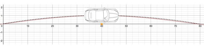
Figure 1- 80′ Slalom Paths

I’ve done the calculations and can tell you that, assuming circular arcs, my 5th gen Corvette, given the same width and same 2″ distance off the cones as before, cornering at a constant 1.2Gs in a 80′ slalom would travel at 62.3mph and take 0.88 seconds between cones.

Here are the calculated times for different slalom cone spacing for a car the width of the C5:

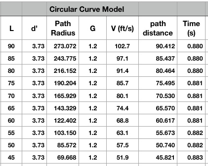
Figure 2- Circular Arc Slalom Times Per Cone

Interesting that the distance between cones makes almost no difference, just as in the sine wave model discussed previously where the difference is zero because distance is not even in the equation. Between 90′ and 45′ the difference is only +/- .001s.

Recall from Transient Response 4 that for a sine curve with a peak of 1.2Gs it should take 0.93 seconds for each cone, not far off what cars regularly achieve and about 6% longer than the times in Figure 2. In Figure 2 the answer does change with distance between cones, if only slightly.

Remember as well that the fastest data for my car at one particular event was 1.05 seconds between cones. I think I’m most interested in the difference between the perfect arc/no transient zone path time of 0.881s (for the slalom spacing in that data) and my actual time of 1.05s. What’s the source of this difference?

Let’s back up and make things clear. The 0.881s time is for a car that has perfect, instantaneous TR, driven perfectly, with perfect balance, etc.  The 1.05s time was as measured in a real, Street-class car (with a real driver of limited skill) that takes time to switch from turning left to turning right and probably never reaches its maximum steady-state lateral G, so it goes slower through the slalom. The relative ability to switch directions is what I think of as Transient Response. So, I think we now have an easy-to-get and real-world-accurate measure of TR for any car.

The measure of TR is then the ratio of how much time a car would take to negotiate each slalom cone if it had infinite TR, given it’s actual maximum lateral cornering capability, to how much time it actually takes. I’ll call this the Slalom Efficiency. In the case of my Corvette it would be

Slalom Efficiency = .881s / 1.05s = 0.84 or 84%

If my car was actually capable of 1.3Gs, as my V-Box said it was reaching, then the Slalom Efficiency is less.  At 1.3Gs I calculate that my car should pass each cone in only 0.846s, given perfectly circular arcs, so the new efficiency is:

Slalom Efficiency (for 1.3Gs) = .846s / 1.05s = .81 or 81%

For the Street Prepared car whose data showed it reaching only 1.2G steady-state, but consistently reaching this level in the slalom and taking just less than 1s, let’s say it was 0.98s, its efficiency on that day on that course with that driver was:

Slalom Efficiency (SP car) = 0.881s / 0.98s = .90 or 90%

The more time a car can spend in a slalom carving a circular arc (at its maximum lateral capability) the higher its Slalom Efficiency will be. Only fast TR allows reaching and/or spending any significant time at max Lateral G around each cone. That’s why Slalom Efficiency is a good measure of transient response.

We can easily rate any car for transient response by finding its Slalom Efficiency.  Many autocrossers already have the data they need for their own car. For more perfect data we need only install a data-device (even a 10hz GPS-only device should work fine) and run it through two exercises: 1) a 200′ skidpad and 2) a longish slalom. Run the car on the skid pad to find its steady-state lateral G capability and then run it in the slalom and find the average time between cones. Plug in the numbers and produce a Slalom Efficiency percentage. A car with infinite transient response, perfectly driven and with perfect balance, would score 100%. All real cars (with real drivers) will score less.