Recap from Part 1
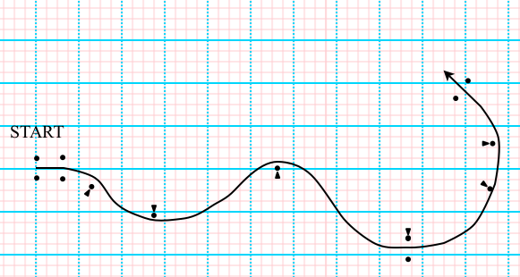
To recap and clarify, I’m attempting to determine whether and how the proper radius around an offset cone changes with the acceleration capability of the car. The objective, as always in this blog, is to learn how to Save Time. A series of offset cones and the way I usually drive it looks like this:

Setup
The situation I’m modeling, with the aid of spreadsheet math and some graphical solutions, is an endless progression of offset cones with, theoretically, a 90 degree turn required at each cone. (In reality, the turns have to be more than 90 degrees.) The finish is not in play and I’m not discussing cornering techniques, per se. (If you want to see what I think about cornering techniques, see previous post All Those Books On Cornering are Wrong.) To be clear, what I’m going to show is NOT considered by me to be the best way to take a corner.
The figure below shows the area of analysis, namely the 150′ before any particular cone and 75′ after it:

I assume, for ease of calculation and graphics, that we go wide on the entry, brake down to the curve velocity the tires can handle, and execute the turn before reaching the cone. Sort of like back-siding the cones in a slalom. (This is simplified as compared to advanced cornering techniques, but I think it will be useful. And, best of all, I can calculate the heck out of it.) Once alongside the cone the car then accelerates at full and constant capability for 75 feet further. The specific area of analysis and various possible paths are shown in the next figure, repeated from Part 1:

Diagram of the Specific Area of Analysis
Calculations
I’m now going to discuss how the calculations are done. Those not interested can skip down to the results. Go on ahead. I won’t be offended.
First, I choose a radius for the turn. Given the 1.2G lateral capability assumed for all cars, physics sets the speed in the arc.
I graphically set the tangent point from the approach and determine the arc distance. Then I calculate the time spent in the curve, which is at a constant velocity. (All calculations use the standard equations of motion I learned a long time ago, forgot for many years and had to re-learn. Far as I know they haven’t changed too much.) From here I can go both forward and backward to determine the remaining segment times.
Since I know the speed in the curve and the acceleration capability of the car, I can easily calculate the time to accelerate through the 75 feet and the speed at the exit. So, yeah, I do that.
Here’s where I have to take the teensiest of short-cuts: I assume a constant entry speed, starting at A in the figure above, of 50 mph. The beauty of this is that now I can easily calculate the distance needed to slow the car from the set 50 mph down to the arc speed given a 1.0G braking capability. (If I don’t make the constant entry speed assumption, this gets too tough for my brain and my spreadsheet.) It’s then not hard to determine the time to cover that distance, figure out how far the car traveled at 50 mph and calculate that segment time as well. Add all the segments times together and you get the time from entry to exit, A to C.
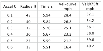
Here’s a picture (probably unreadable) of the spreadsheet. In the upper right corner, in the red box, is the acceleration capability that can be varied. This shot shows 0.4 g. As it changes, the various columns of figures change. Each column starts with a different arc radius, from 5′ to 55′. All velocities are in feet per second in the spreadsheet.

Spreadsheet Data for 0.4G Acceleration Capability
There will be one number in the Total Time row near the bottom in the figure above that is a minimum. In this case, it’s 5.674 seconds and it corresponds to a 30′ arc radius, both values in red boxes. So, now I know that for a 0.4g car a 30′ radius is best, i.e. Saves The Most Time.
Results
I’ve worked the spreadsheet and the graphics from 0.1g to 0.6g and converted the velocities to miles per hour. The results are below.
Best Corner Radii per Acceleration
Hmm. Take a look at those curve velocities. More on that in a sec.
Here is what the three radii, 25′, 35’and 45′ look like with 150′ from A to B:
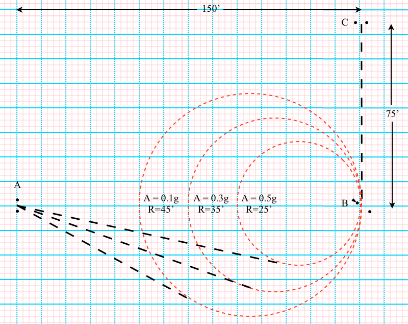
Example Result Paths
Conclusions
- Hey, the standard wisdom is right! The slower-accelerating the car the bigger the radius you should take. Holy Toledo Pro-Solo!
- I’m a little surprised by how big the radii are., i.e. how far outside the cone you have to aim. This says I’ve been driving too tight.
- I find it interesting that the time for a 0.2g HS econobox is not really that much slower than a 0.6g STU Corvette.
- Some of these radius speeds are really too low. The 0.6g car is only going 16.4 mph around the 15′ arc. Even for such a powerful car, in reality it will lose too much time trying to accelerate in 2nd gear from this speed. For most engines the RPM will be too low in 2nd gear. If we set a lower bound on the curve speed of 25 mph to keep from having to downshift this would limit almost all cars to no less than a 35′ radius. I almost never see people in powerful cars taking such big radii. What gives? Some factor I’m missing, maybe? Maybe a sliding, trail-braked, decreasing radius arc just looks a lot different and gives the impression of a tighter radius.
Sensitivity
One last thing: how sensitive is the data? What I mean is, how close to the theoretically right radius do you need to be? The answer is: not very. This is good news, especially for me and my driving!
If you take a look at the Spreadsheet Data for 0.4G figure, the time difference between the perfect radius of 30′ and plus or minus 5′ radius on either side is only 0.005 seconds either way. Given that, the difference in acceleration available at the cone from taking a bit larger radius than theoretically optimum could be significant. So, looks like it would always be better to go a little big. This means I’ve really been driving too tight. The difference in initial acceleration in my BS Corvette from between 21 mph and 25 mph is significant.
Whew! I’ve been working on the subject of these two posts for a long time. Glad it’s done. Please let me know if you find any errors.