Note: A mistake in my calculations was pointed out to me by the observant S. J. Fehr. I pulled this post down for a while and fixed it. I apologize to those that read it earlier.

Now I’d like to assume a different, very simple, path model for a car transiting a slalom. Not because it’s necessarily more accurate than the sine curve but because it will be useful.

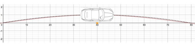
Let’s assume a car has infinite Transient Response (TR). Such a car could switch from turning left at max lateral-G to turning right at max lateral-G in no time at all. The path for such a car in a slalom would be a series of back to back circular arcs. Overlaid on the previous picture of a sine curve it would look like this where the two curves are almost, but not quite, the same. The red is the sine curve and the black is a circular arc.

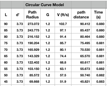
I’ve done the calculations and can tell you that, assuming circular arcs, my 5th gen Corvette, given the same width and same 2″ distance off the cones as before, cornering at a constant 1.2Gs in a 80′ slalom would travel at 62.3mph and take 0.88 seconds between cones.

Here are the calculated times for different slalom cone spacing for a car the width of the C5:

Interesting that the distance between cones makes almost no difference, just as in the sine wave model discussed previously where the difference is zero because distance is not even in the equation. Between 90′ and 45′ the difference is only +/- .001s.

Recall from Transient Response 4 that for a sine curve with a peak of 1.2Gs it should take 0.93 seconds for each cone, not far off what cars regularly achieve and about 6% longer than the times in Figure 2. In Figure 2 the answer does change with distance between cones, if only slightly.

Remember as well that the fastest data for my car at one particular event was 1.05 seconds between cones. I think I’m most interested in the difference between the perfect arc/no transient zone path time of 0.881s (for the slalom spacing in that data) and my actual time of 1.05s. What’s the source of this difference?

Let’s back up and make things clear. The 0.881s time is for a car that has perfect, instantaneous TR, driven perfectly, with perfect balance, etc.  The 1.05s time was as measured in a real, Street-class car (with a real driver of limited skill) that takes time to switch from turning left to turning right and probably never reaches its maximum steady-state lateral G, so it goes slower through the slalom. The relative ability to switch directions is what I think of as Transient Response. So, I think we now have an easy-to-get and real-world-accurate measure of TR for any car.

The measure of TR is then the ratio of how much time a car would take to negotiate each slalom cone if it had infinite TR, given it’s actual maximum lateral cornering capability, to how much time it actually takes. I’ll call this the Slalom Efficiency. In the case of my Corvette it would be

Slalom Efficiency = .881s / 1.05s = 0.84 or 84%

If my car was actually capable of 1.3Gs, as my V-Box said it was reaching, then the Slalom Efficiency is less.  At 1.3Gs I calculate that my car should pass each cone in only 0.846s, given perfectly circular arcs, so the new efficiency is:

Slalom Efficiency (for 1.3Gs) = .846s / 1.05s = .81 or 81%

For the Street Prepared car whose data showed it reaching only 1.2G steady-state, but consistently reaching this level in the slalom and taking just less than 1s, let’s say it was 0.98s, its efficiency on that day on that course with that driver was:

Slalom Efficiency (SP car) = 0.881s / 0.98s = .90 or 90%

The more time a car can spend in a slalom carving a circular arc (at its maximum lateral capability) the higher its Slalom Efficiency will be. Only fast TR allows reaching and/or spending any significant time at max Lateral G around each cone. That’s why Slalom Efficiency is a good measure of transient response.

We can easily rate any car for transient response by finding its Slalom Efficiency.  Many autocrossers already have the data they need for their own car. For more perfect data we need only install a data-device (even a 10hz GPS-only device should work fine) and run it through two exercises: 1) a 200′ skidpad and 2) a longish slalom. Run the car on the skid pad to find its steady-state lateral G capability and then run it in the slalom and find the average time between cones. Plug in the numbers and produce a Slalom Efficiency percentage. A car with infinite transient response, perfectly driven and with perfect balance, would score 100%. All real cars (with real drivers) will score less.

Note: An error in how I calculated d in the equations herein was pointed out to me. I revised this post accordingly within a few hours of initial publication.

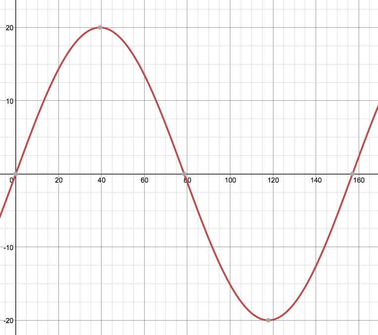
The model of a car negotiating a slalom that produced the equation T = (pi/8) x (d/G)^0.5 in CVD5 is based on the math of a sine curve which looks like this, which is the curve for y = 1sin(0.04x):

Hey, this looks like an overhead view of a car negotiating an 80′ slalom, doesn’t it?

We can even add cones and little picture of car and, wow, this must be a good model of what really happens, right? I mean, doesn’t it look right?

Maybe not.

The first thing that bothers me about this picture of a sine wave is the way the change in direction occurs very smoothly and slowly along the path. This makes it look like there’s plenty of time and space to effect the transient from one direction to another, the center of which, the way I’ve drawn it (but maybe not how you’d drive it) is where the path crosses the horizontal axis. It makes it looks like transient response (TR) isn’t important. In reality I know that to go fast in a slalom in my Street class Corvette, or my Street class Porsche 944, or even in the Porsche Cayman I co-drove recently, I must turn the wheel absolutely as fast as humanly possible and then wait on the car to turn and develop peak lateral capability in the new direction. Then I have to again turn the wheel back the other way as fast as possible and very early or I’ll get late and my line will deteriorate until I hit a cone. Hmmm.

We’ll get back to this question of whether the sine curve is actually a good model a little later.

For now, let’s look at this expression T = (pi/8) x (d/G)^0.5  where T is the time between cones in seconds, d is the lateral distance to the outside edge of each car on each side of the path in feet that the car has to travel to miss the cones and G is the peak lateral acceleration of the car in gravitational units where the force of gravity on the surface of the earth is 1.00 G.

Notice that the distance between cones is not to be found in the equation.

Go ahead, look at it again to make sure. I’ll wait.

This tells us that the distance between cones is either of zero importance or not very important. We can’t really tell which it is because it might be a result of a simplification and I don’t have the original derivation to look at. We are going to have to trust that any such simplification was justified. If you think about it, it makes a certain sense: as the cones get farther apart the car can go faster and the time might just stay the same. Or pretty close to the same.

I’ve worked an example: My corvette is 73.6″ wide. Let’s say I drive 2″ away from the 12″ wide base of the slalom cones. d in the equation is then 12″/2 + 2″ + 73.6″ = 81.6″ which is 6.8 feet. My car easily pulls 1.2Gs in a sweeper. Plugging these values into the equation gives a time T of 0.935 seconds.

Is this number of 0.935 seconds in the ball-park of being correct? I’ve taken a lot of data on my car and, while reasonably close, I never do slaloms that fast. It takes longer, over a full second. I might not be consistently 2″ off the cones but I’m close.

So I went back to find some recent data. Here are some slalom average peak to peak times in my B-Street Corvette from four different runs at an event with a 5 cone slalom consistently spaced at about 75 feet: 1.12s, 1.11s, 1.11s, 1.05s. (Each of these values is the average over 4 peaks within a single, long slalom.) Now if there’s one thing a GPS device knows accurately it’s time of day and time between events. The speed of the car was very consistent from entry to exit. (Luckily, there wasn’t an acceleration zone at the exit.) The last and fastest number happened to be my last and fastest run in the best conditions.

Using that last, fastest number of 1.05s and back-plugging into the formula indicates a lateral G of 0.95G. Peak G in a sweeper was consistently recorded at 1.3G by my 20Hz V-box, but peak G in the slalom was recorded as only 0.55G. So, while the V-box is missing the peaks in the slalom my car is still not achieving it’s steady-state lateral G peak in a slalom, based on the time between cones. I’m not reaching 1.3G in the slalom. I’m not reaching 1.2G in the slalom. I’m not even reaching 1.0G in the slalom.

Some will, of course, say that I just can’t slalom worth a damn. Maybe, but I don’t think that’s it. I think it’s because I can’t change direction fast enough. (Yes, I’m blaming the car!)

This brings me to a key point: Many people look at the sine curve equation and come to the conclusion that if they make their car capable of cornering harder then they’ll be able to go through a slalom faster.

Even if this equation is more or less correct it doesn’t say that. Let me repeat: it does not say that.

What it says is that if you know the peak lateral g a car actually reaches in a slalom and you assume a sine curve path then you can calculate the theoretical time it takes to go from one cone to another.

Two key assumptions are at work here and we need to examine each of them.

1) the car follows a sine curve path

2) the car can change direction (transition) fast enough that the car can reach it’s peak lateral G capability before it’s time to turn the other way.

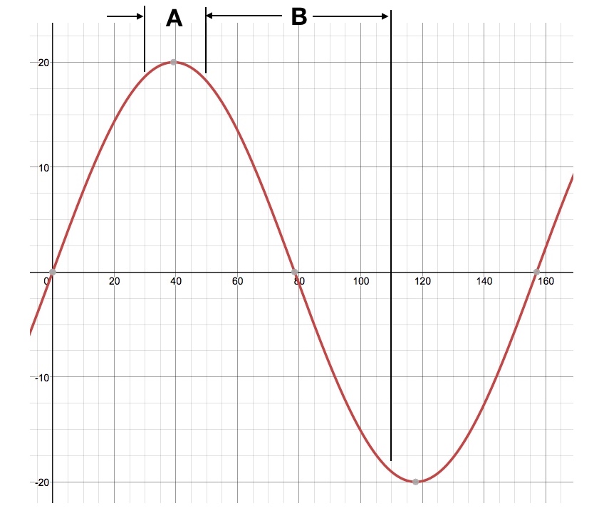
What if neither of these is true? Let’s look at the sine wave path again. Here’s another one for y = 20sin(.04x):

We don’t drive slaloms like that, of course, but if we really wanted to make sure we reached maximum lateral G in each turn we could trade d for G or even velocity for G. This reminds me that we need to be cautious when we look at slalom data because some people (usually novices) do versions of exactly this. They drive farther off the cones and/or slower and wider so they really feel the lateral G at each peak and think they’re driving the car at it’s limits. They’re driving it to some limit, for a moment at least, but clearly not the fastest way through a slalom.

What I notice from looking at this picture is something else. It’s the way the radius of curvature changes. Here it is again with some annotations:

Notice that in the section labeled A the radius of curvature changes very rapidly on either side of the peak. if you start at the peak and then move either left or right the radius changes quickly from max curvature (minimum radius) at the peak to almost a straight line, i.e. a very large radius. Then in the section labeled B, which is most of the time between cones, there’s only a very slow change of radius. That is, the car is essentially driving without turning much at all. This behavior of the sine curve path is always there no matter if it looks like like y=1sin(.04x) in Figures 1 and 2 or y = 20sin(0.04x) just above. Figure 4 only exaggerates the effect. In a sine curve the radius of curvature is increasing non-linearly as it approaches and leaves the peak G point and decreasing non-linearly as it leaves the peak G point. We know this because of the way the path radius changes, given an approximately constant speed.

Is that what happens when we drive a slalom? I don’t think so.

Say you are going straight and suddenly, quickly turn the wheel. You’ve just done a step-steer test. What happens is that the lateral G rises rapidly and almost perfectly linearly. All the step-steer testing results (per ISO 7401) I’ve seen show a rapidly and basically linearly rising G level.

However, these tests are usually limited to only 0.4G to 0.6G. They do this because tires are generally linear in their response up to those levels. After that the tire and suspension bushing non-linearities begin to complicate things.

Us autocrossers don’t do step-steer tests, exactly, anyway. We can add or subtract steering angle as we please to try to get to max lateral G as fast as possible. (The step-steer test turns the wheel once, either by a human or a robot, then holds position.) So, we need to see what a real car with an experienced human driver can do.

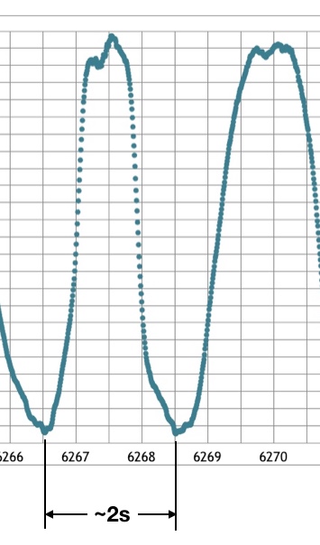
Here’s a graph of the lateral acceleration vs. Time in a slalom of an autocross car at about the Street Prepared level on Hoosiers taken by an accelerometer at over 180Hz.

This is a plot of lateral acceleration, that is, cornering power, not the path of the car like in the previous figures. The peaks are between 1.1G to 1.2G and here the car is traversing the slalom at very slightly less than 1 second per cone. So this is faster than the time for my Corvette that I stated above. I don’t know what kind of surface it was, the temperature, or anything else about the situation where this data was taken.

You’ll have to trust me but the rest of the data shows steady-state peaks essentially the same as these transient peaks. That means that this car was just reaching its maximum lateral-G capability during the slalom. Actually, I’d say this car was more than reaching it’s steady-state peak capability, at least turning one direction, because on one side the G-peaks appear to be flattening out. If the G-peaks flatten, then it means that the G level has become constant. A car turning at a constant G-level is following a circular arc.

I think I need to repeat that: a car turning at a constant G-level is following a circular arc. Right when the sine wave is doing the opposite.

Notice that the initial rise is linear for maybe 2/3rds of the time, then the rate of increase begins to decrease as the cornering limit is approached. I think this is the driver anticipating the limit and doing what he must to not overshoot and lose control. When the wheel is turned back to center (and beyond) the rate of decrease rapidly gets to an essentially linear rate of change which is carried all the way through zero. (There’s no peak of capability to negotiate where you might lose control of the car as the car approaches the zero radius point.) On the other side of zero the lateral Gs climb linearly again until the rate of change begins to decrease as the new limit in the other direction is approached and the driver tries not to overshoot.

What kind of curve has a radius that increases or decreases linearly with length along the path? I’ll give you a hint: it’s not a sine curve and it’s not a circular arc.

It’s an Euler spiral.

I first heard about Euler spirals in Adam Brouillards’ books Perfect Corner 1 and 2 which I talked about here.

A car that never gets to its steady-state cornering limit in a slalom is actually taking the path of a series of Euler spirals set back-to-back. So far I haven’t been able to draw it. (Sorry!)

A car that can reach its steady-state cornering capability within a slalom transitions from an Euler spiral to a circular arc. The driver would attempt to maintain the circular arc until it was time to transition back the other way.  This is, once again, opposite of what is predicted/assumed by the sine wave model. Where the sine wave model says a car is changing radius at a maximal rate a car with fast transient response is doing the opposite and cornering with a constant radius.

Conclusion: The sine-wave model for negotiating a slalom, which has been accepted for going on two decades, was always just plain wrong. It happens to produce an approximate, roughly correct, believable result because the actual path of normal-sized cars in normal-sized slaloms is similar.

The next installment will discuss more about non-sine curve slalom paths and I’ll introduce a testable, standard measure of a car’s slalom efficiency, which will of course be a good measure of transient response, yet not quite the same thing as raw speed through a slalom.

When it comes to transient response many of us have some strange ideas, me included. Let me illustrate this with one true statement and one false statement.

Statement 1:  The polar moment of inertia has a significant effect on how fast a car spins.

     This statement is true.

Statement 2: The polar moment of inertia has a significant effect on transient response.

     This statement is false.

Is the falsity I claim for statement 2 surprising to you? It was to me. I mean, whenever people talk about handling they always say something like a mid-engined car handles quicker and is more responsive because of the lower polar moment than a front engined car.

Witness a 2011 in-depth handling comparison between two Porsches, the Cayman R and the 911GT3, done by Car and Driver here in which the 911GT3 puts the Cayman R to shame. They mention polar moment, Center of Gravity, yaw rate and even a “new step-steering-input maneuver.” New to them, I guess. They ran a variation on ISO 7401 which had been around since 1988 and researchers and car companies had been doing step-steer testing long before it was codified into a standard. Why they couldn’t have just run ISO 7401 (it’s not difficult) I don’t know.

They talk about how the Cayman R’s 20 percent less polar moment of inertia “theoretically [makes] it easier to begin and end any cornering maneuver.” Unfortunately, they don’t actually know what they’re talking about. In fact, they totally miss the point of the step-steer test in my opinion.

Car and Driver does a step-steer test by turning the steering wheel 90 degrees and then reports the final rates at which the two cars turn in degrees per second. Who cares about that? The point of a step-steer test is to determine response time. The time it takes for the car to reach 90% of the final turning rate is the standard result of a step-steer test. That time value is the measure of transient response, not the steady-state turning rate it finally reaches for a given angle of steering input. What they report is really just a simple measure of steering ratio!

I don’t want to pick on Car and Driver too much. The article I’m referencing is not bad, mostly because of the battery of tests they did. They meant well. One test is worth 10 theoretical analyses in my book. I forgive their lack of real car handling engineering knowledge but can’t quite forgive that they don’t go out and find someone (say, any kid who did chassis design in an FSAE program at college) to explain it to them before they write the article and lord theory over us so much. For instance, they conclude that the 0.6″ lower CG height of the GT3 is not nearly as significant as the 20% less polar moment of the Cayman. Really? How do they know? One might ask: if the smaller polar moment is so important, why didn’t the Cayman R do better? Why did the two cars exhibit exactly the same yaw rate of 30 degrees per second if the Cayman has 20% less polar moment?

Seems like that should have been a hint that they weren’t looking at the problem correctly.

Then there’s the fact that the 911 was wearing vastly superior tires than the Cayman which makes the entire set of tests extremely suspect. Couldn’t they have at least put the same tire brand and model on the two cars at the stock widths and eliminated that glaring discrepancy?

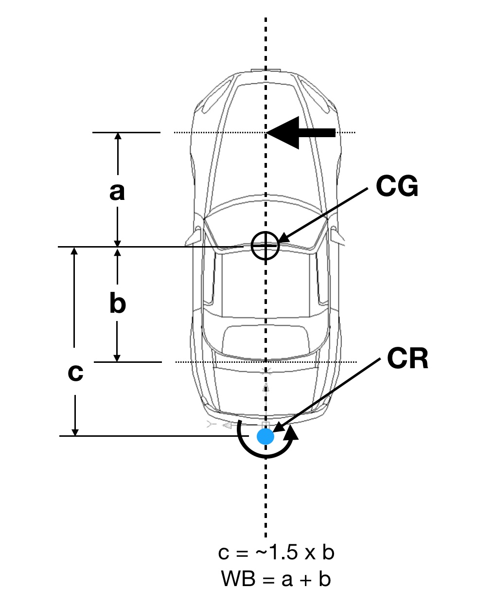
OK, Fisher, if you’re so smart why don’t you tell us what really affects transient response, i.e. step-steer test results? Since you ask, I will, but I’ll need to refer to the following chart.

Here we have a plan view of a car with the Center of Gravity (CG) shown near the center and a big black arrow showing where the initial force comes in from the front wheels to turn the car. The polar moment of inertia would be the sum of all the masses of the car times the square of their distances from the CG. That’s a nice thing to know and it does directly affect how fast the car will rotate once it’s in a spin. The main problem is that when initiating a turn a car does not rotate about the CG.

If the car doesn’t rotate about the CG when a car begins to turn then the polar moment is of minor importance to transient response.

When initiating a turn, say with the ISO 7401 step-steer test, which happens every time a car on a race-track enters a corner from a straight, the car actually rotates about a point that is back behind the rear axle. I have it labeled CR (Center of Rotation.) How far behind the rear axle is it? Using data from testing done by the National Highway Transportation Safety Administration (NHTSA) Bobier, et al, in a 1998 paper entitled Transient Responses of Alternative Vehicle Configurations, found that for 90% of all vehicles tested this point was between 1.39 and 1.96 times the distance from the CG to the rear axle, which is dimension b in the figure above. That puts the CR back behind the rear bumper on most cars just as I’ve drawn it.

So, what we really need to know to estimate transient response is the moment of inertia about point CR, not the (polar) moment of inertia about the CG.

For my purposes I simplify and approximate the location of CR by means of the formula c = 1.5 x b. I’ll call this equation 1.

(At this point anyone who doesn’t want to see how I do this stuff with equations can skip on down to the last equation.)

We can easily determine the value of b for any particular car by finding the wheel-base (WB) and the weight distribution on the internet, which is usually reported by the manufacturer or someone who has measured it.

So, b = WB x (1 – %R)

where WB is the wheelbase and %R is the percentage of weight on the rear axle. Call this equation 2.

Again, what I’m after is an estimate of the yaw inertia about the point CR, not the polar moment inertia about the CG. We can get a good, first-order estimate with this equation

Iy = wt x c^2

where Iy is the yaw inertia, wt is the weight of the car and c is the distance from the CG to the CR.

Now I just substitute equation 2 into equation 1 and take that result and substitute it into equation 3 and we have

Iy = wt x (1.5 x (1-%R) x WB)^2

This gives an estimate of yaw inertia in terms of three parameters that we can fairly easily find for most cars, especially sporty cars.

What does this equation tell us? It tell us that the lower the weight of the car the lower the yaw inertia, all else equal. It tells us that the shorter the wheelbase the lower the yaw inertia, all else equal. And it especially tells us that the further the weight is toward the rear, that is, the closer the mass is to the actual initial center of rotation (not the CG!) the lower the yaw inertia.

Guess what car has a really short wheelbase and has it’s CG way back toward the rear and is only slightly heavier than a Cayman R? A 911GT3, that’s what car.

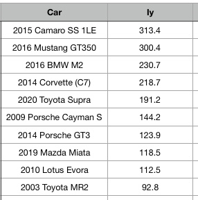
So, a mid-engined car can be expected to have faster response primarily because it will have more weight to the rear, not primarily because it’s weight is centralized. That’s why a front mid-engined car, like the fifth generation Corvette I have, is never going to have the response of a Porsche Cayman, even though its polar moment might be exactly the same. The mid-engined Lotus Evora has better response than the mid-engined Cayman because it has a weight distribution more rearward, very similar to a 911, in fact, as compared to a Cayman. (The Lotus designers knew what they were doing!) And if you get a car very light, with an extremely short wheelbase and make it mid-engined, well then you have a Toyota MR2 Spyder and when you step into it from your Corvette at the autocross you will run over each and every key cone until you get used to how incredibly fast it turns in!

This is what I use in my autocross speed rating system that some people know about. It gives an idea of the potential that a car has for having rapid transient response. Here are some selected results:

Stay tuned. More to come.